- Overview
- Data types in Vega-Lite
- Using Vega-Lite
- In-class Activity: Making changes yourself
- And beyond
Overview
So far, we have processed and analyzed datasets programmatically, using TypeScript functions to compute summary statistics like average, minums, and maximums. An additional tool in the toolkits for data analysts is data visualization. Data visualization has been used throughout history to help humans explore and explain enormous amounts of data.1
So, in addition to computing numerical statistics, we’ll make use of graphics to help communicate insights from our data. We’ll use Vega-Lite for this purpose. Vega-Lite lets us define fairly complex charts using a very simple syntax of field names and values, i.e., objects.
Data types in Vega-Lite
Just like in TypeScript, it’s important to know the kind of data we’re dealing with, because that dictates what we can (and should) do while make charts based on the data.
You know about TypeScript data types like number, boolean, string, or interfaces you create that are made up of these types.
In Vega-Lite, a similar concept exists. It has its own broader categories of data, described below.
Quantitative data is numerical. It can be used in mathematical calculations; we can do things like calculating the average of a list of quantities. For example, a student’s age or the number of units they are taking are examples of quantitative data.
Nominal data is data that can be labelled or classified into different categories. For example, a student’s major or favourite colour are examples of nominal data. Importantly, there is no order or sequence associated with nominal data. The colour Green doesn’t come before or after the colour Red, and the major Computer Science is not better or worse than the major Palaeontology.
Ordinal data is like nominal data, except that the labels do have natural orderings. For example, months are an example of ordinal data. Terms like January, February, etc. are labels, but there is a natural expected ordering between them. Another example are letter grades (i.e., A, A-, B+, etc.). Importantly, the “distance” between two labels of ordinal data is not known—we can’t calculate the “time difference” between events that occurred in January and February or the difference in score between A and B–scoring students.
Consider the following data, showing the number of CS degrees awarded by Cal Poly each year from 2015 to 2019.
[
  {"year": 2015, "degrees": 121},
  {"year": 2016, "degrees": 144},
  {"year": 2017, "degrees": 177},
  {"year": 2018, "degrees": 175},
  {"year": 2019, "degrees": 186}
]
Each object has a year and a degrees value.
The year is ordinal (even though it looks like a number!).
The degrees value is quantitative.
Why do you suppose we’re thinking of year as ordinal?
Using Vega-Lite
Now that we have some data in hand, let’s start simply. We’ll make a univariate visualization of only one field: the number of degrees awarded (degrees). You can follow along in the online Vega editor. Write your chart specification in the editor pane on the left, and the chart will appear on the right.
Visualizations in Vega-Lite are written as Objects with particular fields.
To create a Vega-Lite visualization, we need to specify the data, a mark, and graphical encodings. The data can be depicted as we’ve seen above, i.e., as an array.
Below, we’ll talk about the mark and graphical encoding.
Mark
A mark is the thing that is drawn to the screen. There are number of mark types available in Vega. Some examples you’re like to use this quarter are: bar, circle, line, point, rect, and text.
But we’ll start with a simple mark: a point. Copy the following into the Vega editor.
(The $schema bit below acts sort of like an “interface” for this chart definition.
It contains information about what fields are expected, allowing the editor to give us useful error messages if we make mistakes.
For example,, we would get a compiler error if we forgot to provide data.
Omitting the $schema won’t cause an error, but it will make debugging more difficult.)
{
  "$schema": "https://vega.github.io/schema/vega-lite/v5.json",
  "data": {
    "values": [
      {"year": 2015, "degrees": 121},
      {"year": 2016, "degrees": 144},
      {"year": 2017, "degrees": 177},
      {"year": 2018, "degrees": 175},
      {"year": 2019, "degrees": 186}
    ]
  },
  "mark": {
    "type": "point"
  }
}
You can additional fields to the "mark" object, e.g., to set its color.
  ...previous stuff stays the same
  "mark": {
    "type": "point",
    "color": "firebrick"
  }
With the code above, we’ve given the chart data and we’ve given it a mark (i.e., a shape to draw). But we haven’t mapped the mark’s position to any specific fields in the data, so all the marks are drawn in the same place.
Since the points are not being spread out, the points just get drawn on top of each other. To us, this appears like one single point was drawn.
Not a very meaningful chart!
What we need is a graphical encoding.
Encodings
A graphical encoding maps individual fields in the data (like degrees, for example) to visual channels.
What’s a visual channel? A visual channel is, simply put, stuff we can see. It is a way to control the appearance of marks in a data visualization, e.g., a point’s colour, size, or position.
Coming back to our chart, let’s map the position visual channel, specifically, the mark’s horizontal position, to the degrees field. Modify the chart by adding the encoding field as follows:
{
  "$schema": "https://vega.github.io/schema/vega-lite/v5.json",
  "data": {
    "values": [
      {"year": 2015, "degrees": 121},
      {"year": 2016, "degrees": 144},
      {"year": 2017, "degrees": 177},
      {"year": 2018, "degrees": 175},
      {"year": 2019, "degrees": 186}
    ]
  },
  "mark": {
    "type": "point"
  },
  "encoding": {
    "x": {
      "field": "degrees",
      "type": "quantitative"
    }
  }
}
We told the chart to map the field degrees to the x axis (i.e., the horizontal position visual channel).
We should now see the following univariate (single-variable) scatterplot.
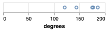
Notice that we specified that the type of data in the degrees field is quantitative.
This means Vega understands that it should treat the values as numbers.
What do you think are the consequences of this?
Specifically, what if we had marked degrees as nominal, or left it blank?
Expand to see the result.
We’d get the following. The degrees values are being treated as *categories* instead of *numbers*, so they’re not being distanced according to their values. Moreover, they're not even in the right order! That’s why its important to be clear about the types of data we’re dealing with at all times.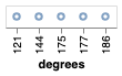
Adding another variable
Let’s add a new dimension to our visualization.
We’ve already given the x channel something to draw, so we can’t give it more to draw.
Note that this is not really a limitation of the computer—the computer can draw pixels on the same position over and over again, like we saw in the first plot we made.
The limitation is with humans—we can’t handle too much information coming into one visual channel.
So here we will add marks to another visual channel—the y axis.
This is simple enough:
{
  "$schema": "https://vega.github.io/schema/vega-lite/v5.json",
  "data": {
    "values": [
      {"year": 2015, "degrees": 121},
      {"year": 2016, "degrees": 144},
      {"year": 2017, "degrees": 177},
      {"year": 2018, "degrees": 175},
      {"year": 2019, "degrees": 186}
    ]
  },
  "mark": {
    "type": "point"
  },
  "encoding": {
    "x": {
      "field": "degrees",
      "type": "quantitative"
    },
    "y": {
      "field": "year",
      "type": "ordinal"
    }
  }
}
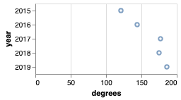
We add in an encoding for the y axis, telling it to plot points based on the year. Notice that we’ve marked the year as an ordinal data type. Please read about the different types of data earlier in this module to remind yourself of why that is.
In-class Activity: Making changes yourself
What we have so far is a scatterplot. These are usually used when we want to plot two quantitative variables. However, here we are plotting one quantitative and one ordinal variable.
Make the following changes to the graph:
- We’d like to plot
barmarks instead ofpointmarks. - In
barcharts, the bars usually go up, not to the right. Change the graph so that the number of degrees is represented by the height of the bars (as opposed to their length).
And beyond
The lab activity that we release today will ask you to create more complex visualizations with Vega-Lite, and make use of additional features such as aggregations.
You strongly encouraged to peruse the Vega-Lite documentation for more ideas and information about how to use the library effectively. In the final project, you will (in teams) be asked to create multiple visualizations using Vega-Lite, and I would love if you explored the documentation and experimented with various visualization types!
-
For example, the earliest navigational maps were examples of data visualization. In the 1800s, the visualization work of John Snow (not that one) helped stop a cholera outbreak. And we’ve already seen Charles Minard’s visualization of Napoleon’s invasion of Russia. ↩